Tracing in OpenGGCM fields#
[1]:
from __future__ import annotations

import numpy as np
import pyvista as pv
import xarray as xr
from scipy import constants

import ggcmpy.tracing


def to_mesh_lines(df):
    positions = df[["x", "y", "z"]].values
    mesh = pv.PolyData(positions)
    lines = pv.lines_from_points(positions)
    return mesh, lines


def plot_trajectory(plotter, df, **kwargs):
    _, lines = to_mesh_lines(df)
    plotter.add_mesh(lines, **kwargs)
Load an actual OpenGGCM dataset#
It’s not from an actually meaningful simulation, but it’ll do for now. The code below loads the data (which was generated with etajout=true), and then rescales to base SI units (FIXME: we should have the option to just trace in the original units).
In addition, it sets the electric field to zero to make things simpler.
[2]:
R_E = 6.371e6  # m

ds = xr.open_dataset(ggcmpy.sample_dir / "test0008.3df.000007")
x, y, z = R_E * ds.x.values, R_E * ds.y.values, R_E * ds.z.values
ds = ds.assign_coords(
    x=("x", x),
    y=("y", y),
    z=("z", z),
    x_nc=("x_nc", 0.5 * (x[1:] + x[:-1])),
    y_nc=("y_nc", 0.5 * (y[1:] + y[:-1])),
    z_nc=("z_nc", 0.5 * (z[1:] + z[:-1])),
)
ds["bx1"] = (("x_nc", "y", "z"), 1e-9 * ds.bx1.values[:-1, :, :])
ds["by1"] = (("x", "y_nc", "z"), 1e-9 * ds.by1.values[:, :-1, :])
ds["bz1"] = (("x", "y", "z_nc"), 1e-9 * ds.bz1.values[:, :, :-1])
ds["ex1"] = (("x", "y_nc", "z_nc"), 0 * ds.eflx.values[:, :-1, :-1])
ds["ey1"] = (("x_nc", "y", "z_nc"), 0 * ds.efly.values[:-1, :, :-1])
ds["ez1"] = (("x_nc", "y_nc", "z"), 0 * ds.eflz.values[:-1, :-1, :])
ds
[2]:
<xarray.Dataset> Size: 48MB
Dimensions:       (x: 128, y: 64, z: 64, x_nc: 127, y_nc: 63, z_nc: 63, time: 1)
Coordinates:
  * time          (time) datetime64[ns] 8B 1967-01-01T00:00:07.130000
  * x             (x) float32 512B -1.911e+08 -1.792e+08 ... 1.808e+09 1.911e+09
  * y             (y) float32 256B -3.186e+08 -2.892e+08 ... 2.892e+08 3.186e+08
  * z             (z) float32 256B -3.186e+08 -2.892e+08 ... 2.892e+08 3.186e+08
  * x_nc          (x_nc) float32 508B -1.851e+08 -1.735e+08 ... 1.86e+09
  * y_nc          (y_nc) float32 252B -3.039e+08 -2.755e+08 ... 3.039e+08
  * z_nc          (z_nc) float32 252B -3.039e+08 -2.755e+08 ... 3.039e+08
Data variables: (12/25)
    bx            (x, y, z) float32 2MB ...
    by            (x, y, z) float32 2MB ...
    bz            (x, y, z) float32 2MB ...
    vx            (x, y, z) float32 2MB ...
    vy            (x, y, z) float32 2MB ...
    vz            (x, y, z) float32 2MB ...
    ...            ...
    xtra2         (x, y, z) float32 2MB ...
    inttime       (time) int64 8B ...
    elapsed_time  (time) float64 8B ...
    ex1           (x, y_nc, z_nc) float32 2MB 0.0 0.0 0.0 0.0 ... -0.0 -0.0 -0.0
    ey1           (x_nc, y, z_nc) float32 2MB 0.0 0.0 0.0 0.0 ... 0.0 0.0 0.0
    ez1           (x_nc, y_nc, z) float32 2MB 0.0 0.0 0.0 0.0 ... -0.0 -0.0 -0.0
Attributes:
run: test0008Trace using the Boris integrator#
That’s pretty much just the same as in the dipole example, but using the OpenGGCM fields.
[3]:
boris = ggcmpy.tracing.BorisIntegrator_f2py(ds, q=-constants.e, m=constants.m_e)
x0 = np.array([-5.0 * R_E, 0, 0])

B_x0 = boris._interpolator.B(x0)
T_e = 1.0 * 1e3 * constants.e  # 1 keV in J
v_e = np.sqrt(2 * T_e / constants.m_e)  # electron thermal speed
v_e *= 100.0

om_ce = np.abs(constants.e) * np.linalg.norm(B_x0) / constants.m_e  # gyrofrequency
r_ce = constants.m_e * v_e / (constants.e * np.linalg.norm(B_x0))  # gyroradius
print(f"B={B_x0} om_ce={om_ce} r_ce={r_ce}")  # noqa: T201

v0 = np.array([0.0, v_e, v_e])  # [m/s]
dt = 2 * np.pi / om_ce / 20
t_max = 500 * 2 * np.pi / om_ce  # [s]

df = boris.integrate(x0, v0, t_max, dt)
df
B=[0.00000000e+00 1.99064813e-16 2.47747835e-07] om_ce=43574.3848688326 r_ce=43042.197072298615
[3]:
| time | x | y | z | vx | vy | vz | |
|---|---|---|---|---|---|---|---|
| 0 | 0.000000 | -31855000.0 | 0.000000 | 0.000000e+00 | 0.000000e+00 | 1.875537e+09 | 1.875537e+09 |
| 1 | 0.000007 | -31857072.0 | 13195.142578 | 1.352346e+04 | -5.749702e+08 | 1.784837e+09 | 1.875912e+09 |
| 2 | 0.000014 | -31863088.0 | 25114.351562 | 2.705193e+04 | -1.094160e+09 | 1.521589e+09 | 1.876929e+09 |
| 3 | 0.000022 | -31872466.0 | 34606.066406 | 4.058892e+04 | -1.507335e+09 | 1.111443e+09 | 1.878275e+09 |
| 4 | 0.000029 | -31884298.0 | 40754.703125 | 5.413516e+04 | -1.774739e+09 | 5.942084e+08 | 1.879494e+09 |
| ... | ... | ... | ... | ... | ... | ... | ... |
| 9997 | 0.072074 | -25325260.0 | -433478.218750 | -1.013405e+07 | 8.069608e+08 | 1.252936e+09 | 2.194149e+09 |
| 9998 | 0.072081 | -25321328.0 | -420595.406250 | -1.012162e+07 | 2.842814e+08 | 2.320795e+09 | 1.252365e+09 |
| 9999 | 0.072089 | -25321826.0 | -402791.875000 | -1.011731e+07 | -4.223673e+08 | 2.617960e+09 | -5.669133e+07 |
| 10000 | 0.072096 | -25327236.0 | -385979.031250 | -1.012220e+07 | -1.078690e+09 | 2.045977e+09 | -1.298356e+09 |
| 10001 | 0.072103 | -25336414.0 | -375734.250000 | -1.013431e+07 | -1.467493e+09 | 7.959528e+08 | -2.061127e+09 |
10002 rows × 7 columns
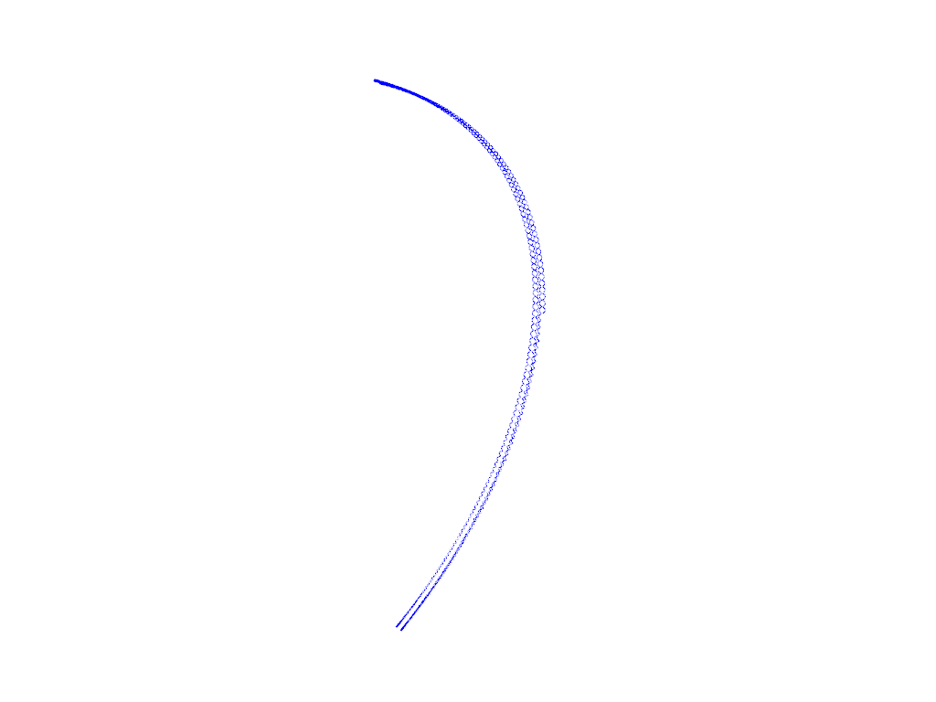
Plot the trajectory#
Not all that exciting, but at least it looks reasonable…
[4]:
plotter = pv.Plotter()
plot_trajectory(plotter, df, line_width=1, color="blue")
plotter.show()
2026-01-15 06:02:05.279 (   1.534s) [    743412AEBB80]vtkXOpenGLRenderWindow.:1458  WARN| bad X server connection. DISPLAY=
/home/docs/checkouts/readthedocs.org/user_builds/ggcmpy/envs/pr-tracing/lib/python3.12/site-packages/pyvista/jupyter/notebook.py:56: UserWarning: Failed to use notebook backend:

No module named 'trame'

Falling back to a static output.
  warnings.warn(
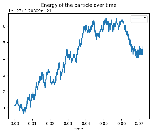
Check energy conservation#
Looks pretty good – the tracing here is done in Fortran with single precision, so a relative error of \(10^{-6}\) is expected due to machine precision.
[5]:
df["E"] = 0.5 * constants.m_e * np.linalg.norm(df[["vx", "vy", "vz"]].values, axis=1)
df.plot(x="time", y="E", title="Energy of the particle over time");