Quick Overview

We’ll import xarray with its standard short name xr, since that’s what we’re using to interact with the data.

ggcmpy is only needed to get access to some sample data.

from __future__ import annotations

import xarray as xr

import ggcmpy

Opening a dataset

Let’s open a sample dataset, in this case it’s a py_0 OpenGGCM output, that is a cut through the 3-d MHD data at position \(y = 0\). Xarray provides a nice summary of the various parts of this dataset – in particular, the dimensions, the coordinates and the various fields (“Data variables”) contained in this file.

ds_py = xr.open_dataset(ggcmpy.sample_dir / "sample_jrrle.py_0.001200")
ds_py

<xarray.Dataset> Size: 115kB
Dimensions:       (x: 64, z: 32, y: 1, time: 1)
Coordinates:
  * x             (x) float32 256B -30.0 -28.8 -27.61 ... 73.25 81.63 90.0
  * y             (y) float64 8B 0.0
  * z             (z) float32 128B -50.0 -40.94 -33.05 ... 33.05 40.94 50.0
  * time          (time) datetime64[ns] 8B 1967-01-01T00:20:00.033000
Data variables: (12/16)
    bx            (x, z) float32 8kB ...
    by            (x, z) float32 8kB ...
    bz            (x, z) float32 8kB ...
    vx            (x, z) float32 8kB ...
    vy            (x, z) float32 8kB ...
    vz            (x, z) float32 8kB ...
    ...            ...
    xjy           (x, z) float32 8kB ...
    xjz           (x, z) float32 8kB ...
    xtra1         (x, z) float32 8kB ...
    xtra2         (x, z) float32 8kB ...
    inttime       (time) int64 8B ...
    elapsed_time  (time) float64 8B ...
Attributes:
    run:      sample_jrrle

xarray.Dataset

• Dimensions:
  • x: 64
  • z: 32
  • y: 1
  • time: 1
• Coordinates: (4)
  • x
    (x)
    float32
    -30.0 -28.8 -27.61 ... 81.63 90.0

    units :

    RE

    long_name :

    -GSE_x

    array([-3.000000e+01, -2.880391e+01, -2.760781e+01, -2.641171e+01,
           -2.521562e+01, -2.401953e+01, -2.282343e+01, -2.162734e+01,
           -2.043124e+01, -1.923515e+01, -1.803905e+01, -1.684296e+01,
           -1.564686e+01, -1.445077e+01, -1.325467e+01, -1.205858e+01,
           -1.086248e+01, -9.666403e+00, -8.477365e+00, -7.342983e+00,
           -6.350031e+00, -5.568631e+00, -4.953945e+00, -4.433165e+00,
           -3.967671e+00, -3.535115e+00, -3.121500e+00, -2.717732e+00,
           -2.318041e+00, -1.919303e+00, -1.520604e+00, -1.121906e+00,
           -7.232079e-01, -3.245094e-01,  7.418892e-02,  4.728872e-01,
            8.715854e-01,  1.270284e+00,  1.668982e+00,  2.067680e+00,
            2.466456e+00,  2.865999e+00,  3.267992e+00,  3.675195e+00,
            4.091593e+00,  4.522704e+00,  4.976123e+00,  5.462518e+00,
            5.997422e+00,  6.604670e+00,  7.323482e+00,  8.224792e+00,
            9.455503e+00,  1.139296e+01,  1.543052e+01,  2.301989e+01,
            3.139135e+01,  3.976402e+01,  4.813668e+01,  5.650934e+01,
            6.488200e+01,  7.325467e+01,  8.162733e+01,  9.000000e+01],
          dtype=float32)

  • y
    (y)
    float64
    0.0

    units :

    RE

    long_name :

    GSE_y

    array([0.])

  • z
    (z)
    float32
    -50.0 -40.94 -33.05 ... 40.94 50.0

    units :

    RE

    long_name :

    GSE_z

    array([-50.      , -40.939518, -33.046852, -26.241549, -20.443153, -15.571257,
           -11.545485,  -8.285531,  -5.711199,  -3.742462,  -2.299564,  -1.303101,
            -0.673488,  -0.3263  ,  -0.156689,  -0.050028,   0.050028,   0.156689,
             0.3263  ,   0.673488,   1.303101,   2.299564,   3.742462,   5.711199,
             8.285531,  11.545485,  15.571257,  20.443153,  26.241549,  33.046852,
            40.939518,  50.      ], dtype=float32)

  • time
    (time)
    datetime64[ns]
    1967-01-01T00:20:00.033000

    array(['1967-01-01T00:20:00.033000000'], dtype='datetime64[ns]')

• Data variables: (16)
  • bx
    (x, z)
    float32
    ...

    shape :

    (64, 32)

    varname :

    bx

    inttime :

    1200

    timestr :

    time= 1200.0 0.315372000332031E+08 1967:01:01:00:20:00.033 c300

    file_position :

    0

    elapsed_time :

    1200.0

    units :

    nT

    long_name :

    magnetic field, x-component

    [2048 values with dtype=float32]

  • by
    (x, z)
    float32
    ...

    shape :

    (64, 32)

    varname :

    by

    inttime :

    1200

    timestr :

    time= 1200.0 0.315372000332031E+08 1967:01:01:00:20:00.033 c300

    file_position :

    3860

    elapsed_time :

    1200.0

    units :

    nT

    long_name :

    magnetic field, y-component

    [2048 values with dtype=float32]

  • bz
    (x, z)
    float32
    ...

    shape :

    (64, 32)

    varname :

    bz

    inttime :

    1200

    timestr :

    time= 1200.0 0.315372000332031E+08 1967:01:01:00:20:00.033 c300

    file_position :

    7860

    elapsed_time :

    1200.0

    units :

    nT

    long_name :

    magnetic field, z-component

    [2048 values with dtype=float32]

  • vx
    (x, z)
    float32
    ...

    shape :

    (64, 32)

    varname :

    vx

    inttime :

    1200

    timestr :

    time= 1200.0 0.315372000332031E+08 1967:01:01:00:20:00.033 c300

    file_position :

    10816

    elapsed_time :

    1200.0

    units :

    km/s

    long_name :

    plasma velocity, x-component

    [2048 values with dtype=float32]

  • vy
    (x, z)
    float32
    ...

    shape :

    (64, 32)

    varname :

    vy

    inttime :

    1200

    timestr :

    time= 1200.0 0.315372000332031E+08 1967:01:01:00:20:00.033 c300

    file_position :

    13418

    elapsed_time :

    1200.0

    units :

    km/s

    long_name :

    plasma velocity, y-component

    [2048 values with dtype=float32]

  • vz
    (x, z)
    float32
    ...

    shape :

    (64, 32)

    varname :

    vz

    inttime :

    1200

    timestr :

    time= 1200.0 0.315372000332031E+08 1967:01:01:00:20:00.033 c300

    file_position :

    17298

    elapsed_time :

    1200.0

    units :

    km/s

    long_name :

    plasma velocity, z-component

    [2048 values with dtype=float32]

  • rr
    (x, z)
    float32
    ...

    shape :

    (64, 32)

    varname :

    rr

    inttime :

    1200

    timestr :

    time= 1200.0 0.315372000332031E+08 1967:01:01:00:20:00.033 c300

    file_position :

    21047

    elapsed_time :

    1200.0

    units :

    1/cm^3

    long_name :

    plasma number density

    [2048 values with dtype=float32]

  • pp
    (x, z)
    float32
    ...

    shape :

    (64, 32)

    varname :

    pp

    inttime :

    1200

    timestr :

    time= 1200.0 0.315372000332031E+08 1967:01:01:00:20:00.033 c300

    file_position :

    23681

    elapsed_time :

    1200.0

    units :

    pPa

    long_name :

    plasma pressure

    [2048 values with dtype=float32]

  • resis
    (x, z)
    float32
    ...

    shape :

    (64, 32)

    varname :

    resis

    inttime :

    1200

    timestr :

    time= 1200.0 0.315372000332031E+08 1967:01:01:00:20:00.033 c300

    file_position :

    26763

    elapsed_time :

    1200.0

    units :

    Ohm m

    long_name :

    plasma resistivity

    [2048 values with dtype=float32]

  • xjx
    (x, z)
    float32
    ...

    shape :

    (64, 32)

    varname :

    xjx

    inttime :

    1200

    timestr :

    time= 1200.0 0.315372000332031E+08 1967:01:01:00:20:00.033 c300

    file_position :

    27524

    elapsed_time :

    1200.0

    units :

    uA/m^2

    long_name :

    current density, x-component

    [2048 values with dtype=float32]

  • xjy
    (x, z)
    float32
    ...

    shape :

    (64, 32)

    varname :

    xjy

    inttime :

    1200

    timestr :

    time= 1200.0 0.315372000332031E+08 1967:01:01:00:20:00.033 c300

    file_position :

    31406

    elapsed_time :

    1200.0

    units :

    uA/m^2

    long_name :

    current density, y-component

    [2048 values with dtype=float32]

  • xjz
    (x, z)
    float32
    ...

    shape :

    (64, 32)

    varname :

    xjz

    inttime :

    1200

    timestr :

    time= 1200.0 0.315372000332031E+08 1967:01:01:00:20:00.033 c300

    file_position :

    35076

    elapsed_time :

    1200.0

    units :

    uA/m^2

    long_name :

    current density, z-component

    [2048 values with dtype=float32]

  • xtra1
    (x, z)
    float32
    ...

    shape :

    (64, 32)

    varname :

    xtra1

    inttime :

    1200

    timestr :

    time= 1200.0 0.315372000332031E+08 1967:01:01:00:20:00.033 c300

    file_position :

    38944

    elapsed_time :

    1200.0

    [2048 values with dtype=float32]

  • xtra2
    (x, z)
    float32
    ...

    shape :

    (64, 32)

    varname :

    xtra2

    inttime :

    1200

    timestr :

    time= 1200.0 0.315372000332031E+08 1967:01:01:00:20:00.033 c300

    file_position :

    39481

    elapsed_time :

    1200.0

    [2048 values with dtype=float32]

  • inttime
    (time)
    int64
    ...

    [1 values with dtype=int64]

  • elapsed_time
    (time)
    float64
    ...

    [1 values with dtype=float64]

• Indexes: (4)
  • x
    PandasIndex

    PandasIndex(Index([              -30.0, -28.803905487060547, -27.607810974121094,
           -26.411714553833008, -25.215620040893555,   -24.0195255279541,
            -22.82343101501465, -21.627336502075195,  -20.43124008178711,
           -19.235145568847656, -18.039051055908203,  -16.84295654296875,
            -15.64686107635498, -14.450766563415527, -13.254671096801758,
           -12.058576583862305, -10.862481117248535,  -9.666402816772461,
            -8.477364540100098,  -7.342983245849609,  -6.350030899047852,
            -5.568631172180176,  -4.953944683074951,  -4.433164596557617,
           -3.9676711559295654, -3.5351150035858154, -3.1215004920959473,
           -2.7177324295043945, -2.3180408477783203, -1.9193027019500732,
           -1.5206044912338257, -1.1219062805175781, -0.7232078909873962,
           -0.3245093524456024, 0.07418891787528992, 0.47288718819618225,
            0.8715854287147522,  1.2702836990356445,   1.668981909751892,
            2.0676803588867188,   2.466456413269043,  2.8659989833831787,
            3.2679920196533203,    3.67519474029541,   4.091593265533447,
             4.522703647613525,   4.976123332977295,   5.462517738342285,
             5.997421741485596,    6.60467004776001,   7.323481559753418,
              8.22479248046875,   9.455503463745117,  11.392964363098145,
             15.43051528930664,  23.019893646240234,    31.3913516998291,
            39.764015197753906,   48.13667678833008,  56.509342193603516,
             64.88200378417969,   73.25466918945312,   81.62733459472656,
                          90.0],
          dtype='float32', name='x'))

  • y
    PandasIndex

    PandasIndex(Index([0.0], dtype='float64', name='y'))

  • z
    PandasIndex

    PandasIndex(Index([                -50.0,   -40.939517974853516,   -33.046852111816406,
             -26.241548538208008,   -20.443153381347656,   -15.571256637573242,
              -11.54548454284668,    -8.285531044006348,   -5.7111992835998535,
              -3.742462158203125,   -2.2995643615722656,   -1.3031009435653687,
             -0.6734877824783325,  -0.32629987597465515,  -0.15668930113315582,
           -0.050028134137392044,  0.050028134137392044,   0.15668930113315582,
             0.32629987597465515,    0.6734877824783325,    1.3031009435653687,
              2.2995643615722656,     3.742462158203125,    5.7111992835998535,
               8.285531044006348,     11.54548454284668,    15.571256637573242,
              20.443153381347656,    26.241548538208008,    33.046852111816406,
              40.939517974853516,                  50.0],
          dtype='float32', name='z'))

  • time
    PandasIndex

    PandasIndex(DatetimeIndex(['1967-01-01 00:20:00.033000'], dtype='datetime64[ns]', name='time', freq=None))

• Attributes: (1)

  run :

  sample_jrrle

Accessing a field

Accessing a particular field (or coordinate) is as simple as ds_py["rr"] for the rr (density) field – a xr.Dataset behaves like a Python dict.

One can even save oneself typing the brackets and quotes, since xr.Dataset also provides access to the variables (fields/coordinates) as attributes, that is, ds_py.rr.

rr = ds_py.rr
rr

<xarray.DataArray 'rr' (x: 64, z: 32)> Size: 8kB
[2048 values with dtype=float32]
Coordinates:
  * x        (x) float32 256B -30.0 -28.8 -27.61 -26.41 ... 73.25 81.63 90.0
  * z        (z) float32 128B -50.0 -40.94 -33.05 -26.24 ... 33.05 40.94 50.0
Attributes:
    shape:          (64, 32)
    varname:        rr
    inttime:        1200
    timestr:        time=   1200.0    0.315372000332031E+08 1967:01:01:00:20:...
    file_position:  21047
    elapsed_time:   1200.0
    units:          1/cm^3
    long_name:      plasma number density

xarray.DataArray

'rr'

• x: 64
• z: 32

• ...

  [2048 values with dtype=float32]

• Coordinates: (2)
  • x
    (x)
    float32
    -30.0 -28.8 -27.61 ... 81.63 90.0

    units :

    RE

    long_name :

    -GSE_x

    array([-3.000000e+01, -2.880391e+01, -2.760781e+01, -2.641171e+01,
           -2.521562e+01, -2.401953e+01, -2.282343e+01, -2.162734e+01,
           -2.043124e+01, -1.923515e+01, -1.803905e+01, -1.684296e+01,
           -1.564686e+01, -1.445077e+01, -1.325467e+01, -1.205858e+01,
           -1.086248e+01, -9.666403e+00, -8.477365e+00, -7.342983e+00,
           -6.350031e+00, -5.568631e+00, -4.953945e+00, -4.433165e+00,
           -3.967671e+00, -3.535115e+00, -3.121500e+00, -2.717732e+00,
           -2.318041e+00, -1.919303e+00, -1.520604e+00, -1.121906e+00,
           -7.232079e-01, -3.245094e-01,  7.418892e-02,  4.728872e-01,
            8.715854e-01,  1.270284e+00,  1.668982e+00,  2.067680e+00,
            2.466456e+00,  2.865999e+00,  3.267992e+00,  3.675195e+00,
            4.091593e+00,  4.522704e+00,  4.976123e+00,  5.462518e+00,
            5.997422e+00,  6.604670e+00,  7.323482e+00,  8.224792e+00,
            9.455503e+00,  1.139296e+01,  1.543052e+01,  2.301989e+01,
            3.139135e+01,  3.976402e+01,  4.813668e+01,  5.650934e+01,
            6.488200e+01,  7.325467e+01,  8.162733e+01,  9.000000e+01],
          dtype=float32)

  • z
    (z)
    float32
    -50.0 -40.94 -33.05 ... 40.94 50.0

    units :

    RE

    long_name :

    GSE_z

    array([-50.      , -40.939518, -33.046852, -26.241549, -20.443153, -15.571257,
           -11.545485,  -8.285531,  -5.711199,  -3.742462,  -2.299564,  -1.303101,
            -0.673488,  -0.3263  ,  -0.156689,  -0.050028,   0.050028,   0.156689,
             0.3263  ,   0.673488,   1.303101,   2.299564,   3.742462,   5.711199,
             8.285531,  11.545485,  15.571257,  20.443153,  26.241549,  33.046852,
            40.939518,  50.      ], dtype=float32)

• Indexes: (2)
  • x
    PandasIndex

    PandasIndex(Index([              -30.0, -28.803905487060547, -27.607810974121094,
           -26.411714553833008, -25.215620040893555,   -24.0195255279541,
            -22.82343101501465, -21.627336502075195,  -20.43124008178711,
           -19.235145568847656, -18.039051055908203,  -16.84295654296875,
            -15.64686107635498, -14.450766563415527, -13.254671096801758,
           -12.058576583862305, -10.862481117248535,  -9.666402816772461,
            -8.477364540100098,  -7.342983245849609,  -6.350030899047852,
            -5.568631172180176,  -4.953944683074951,  -4.433164596557617,
           -3.9676711559295654, -3.5351150035858154, -3.1215004920959473,
           -2.7177324295043945, -2.3180408477783203, -1.9193027019500732,
           -1.5206044912338257, -1.1219062805175781, -0.7232078909873962,
           -0.3245093524456024, 0.07418891787528992, 0.47288718819618225,
            0.8715854287147522,  1.2702836990356445,   1.668981909751892,
            2.0676803588867188,   2.466456413269043,  2.8659989833831787,
            3.2679920196533203,    3.67519474029541,   4.091593265533447,
             4.522703647613525,   4.976123332977295,   5.462517738342285,
             5.997421741485596,    6.60467004776001,   7.323481559753418,
              8.22479248046875,   9.455503463745117,  11.392964363098145,
             15.43051528930664,  23.019893646240234,    31.3913516998291,
            39.764015197753906,   48.13667678833008,  56.509342193603516,
             64.88200378417969,   73.25466918945312,   81.62733459472656,
                          90.0],
          dtype='float32', name='x'))

  • z
    PandasIndex

    PandasIndex(Index([                -50.0,   -40.939517974853516,   -33.046852111816406,
             -26.241548538208008,   -20.443153381347656,   -15.571256637573242,
              -11.54548454284668,    -8.285531044006348,   -5.7111992835998535,
              -3.742462158203125,   -2.2995643615722656,   -1.3031009435653687,
             -0.6734877824783325,  -0.32629987597465515,  -0.15668930113315582,
           -0.050028134137392044,  0.050028134137392044,   0.15668930113315582,
             0.32629987597465515,    0.6734877824783325,    1.3031009435653687,
              2.2995643615722656,     3.742462158203125,    5.7111992835998535,
               8.285531044006348,     11.54548454284668,    15.571256637573242,
              20.443153381347656,    26.241548538208008,    33.046852111816406,
              40.939517974853516,                  50.0],
          dtype='float32', name='z'))

• Attributes: (8)

  shape :

  (64, 32)

  varname :

  rr

  inttime :

  1200

  timestr :

  time= 1200.0 0.315372000332031E+08 1967:01:01:00:20:00.033 c300

  file_position :

  21047

  elapsed_time :

  1200.0

  units :

  1/cm^3

  long_name :

  plasma number density

Plotting

A quick way to plot some data is to just call .plot() on it. Xarray will try to make a sensible default plot given the data provided. In particular for 2-d data it’ll make a pseudo-color plot.

Note: I’m transposing the data with .T before plotting, since otherwise the \(x\) and \(z\) axes end up being swapped, which isn’t how we usually like to look at the magnetosphere.

rr.T.plot();

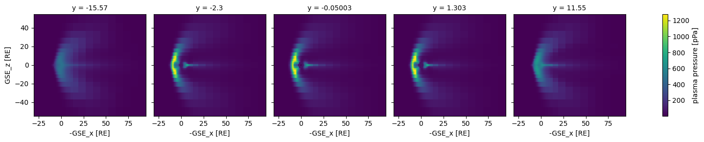
3-d data

Let’s do a bunch of \(x\)-\(z\) plane cuts of the sample 3-d data, showing pressure (pp).

(Note that picking a bunch of times would make more sense, rather than a bunch of \(y\) values, but we only have sample data for a single time.)

ds_3d = xr.open_dataset(ggcmpy.sample_dir / "sample_jrrle.3df.001200")
ds_3d.pp.sel(y=slice(-20, 20, 5)).plot(x="x", y="z", col="y");

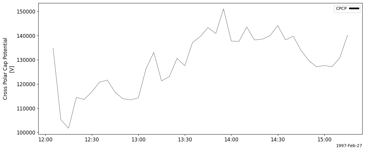
Calculating Cross Polar Cap Potential

import xarray as xr

DATA_DIR = ggcmpy.sample_dir / "cir07_19970227_liang_norcm"
files = sorted(DATA_DIR.glob("*.iof.*"))
iof = xr.open_mfdataset(files)

cpcp = iof.ggcm.cpcp()
cpcp

<xarray.DataArray 'cpcp' (time: 39)> Size: 156B
array([134867.83 , 105205.875, 101696.07 , 114429.28 , 113574.31 ,
       116743.   , 120733.77 , 121602.17 , 116599.71 , 113891.266,
       113451.36 , 114209.516, 126319.875, 133029.05 , 121223.64 ,
       123038.734, 130548.81 , 127525.625, 137121.53 , 139610.44 ,
       143280.47 , 140815.66 , 151007.06 , 137692.9  , 137625.66 ,
       143495.03 , 138163.22 , 138477.53 , 139933.22 , 144133.61 ,
       138196.17 , 139740.44 , 133857.48 , 129707.45 , 127090.39 ,
       127611.05 , 127130.625, 130677.75 , 140149.05 ], dtype=float32)
Coordinates:
  * time     (time) datetime64[ns] 312B 1997-02-27T12:05:00.170000 ... 1997-0...
Attributes:
    long_name:  Cross Polar Cap Potential
    name:       CPCP
    units:      V

xarray.DataArray

'cpcp'

• time: 39

• 1.349e+05 1.052e+05 1.017e+05 ... 1.271e+05 1.307e+05 1.401e+05

  array([134867.83 , 105205.875, 101696.07 , 114429.28 , 113574.31 ,
         116743.   , 120733.77 , 121602.17 , 116599.71 , 113891.266,
         113451.36 , 114209.516, 126319.875, 133029.05 , 121223.64 ,
         123038.734, 130548.81 , 127525.625, 137121.53 , 139610.44 ,
         143280.47 , 140815.66 , 151007.06 , 137692.9  , 137625.66 ,
         143495.03 , 138163.22 , 138477.53 , 139933.22 , 144133.61 ,
         138196.17 , 139740.44 , 133857.48 , 129707.45 , 127090.39 ,
         127611.05 , 127130.625, 130677.75 , 140149.05 ], dtype=float32)

• Coordinates: (1)
  • time
    (time)
    datetime64[ns]
    1997-02-27T12:05:00.170000 ... 1...

    array(['1997-02-27T12:05:00.170000000', '1997-02-27T12:10:00.189000000',
           '1997-02-27T12:15:00.057000000', '1997-02-27T12:20:00.042000000',
           '1997-02-27T12:25:00.095000000', '1997-02-27T12:30:00.109000000',
           '1997-02-27T12:35:00.020000000', '1997-02-27T12:40:00.148000000',
           '1997-02-27T12:45:00.039000000', '1997-02-27T12:50:00.152000000',
           '1997-02-27T12:55:00.002000000', '1997-02-27T13:00:00.135000000',
           '1997-02-27T13:05:00.072000000', '1997-02-27T13:10:00.003000000',
           '1997-02-27T13:15:00.051000000', '1997-02-27T13:20:00.189000000',
           '1997-02-27T13:25:00.056000000', '1997-02-27T13:30:00.015000000',
           '1997-02-27T13:35:00.176000000', '1997-02-27T13:40:00.167000000',
           '1997-02-27T13:45:00.184000000', '1997-02-27T13:50:00.069000000',
           '1997-02-27T13:55:00.148000000', '1997-02-27T14:00:00.161000000',
           '1997-02-27T14:05:00.006000000', '1997-02-27T14:10:00.149000000',
           '1997-02-27T14:15:00.055000000', '1997-02-27T14:20:00.087000000',
           '1997-02-27T14:25:00.072000000', '1997-02-27T14:30:00.097000000',
           '1997-02-27T14:35:00.102000000', '1997-02-27T14:40:00.052000000',
           '1997-02-27T14:45:00.140000000', '1997-02-27T14:50:00.031000000',
           '1997-02-27T14:55:00.108000000', '1997-02-27T15:00:00.185000000',
           '1997-02-27T15:05:00.001000000', '1997-02-27T15:10:00.023000000',
           '1997-02-27T15:15:00.023000000'], dtype='datetime64[ns]')

• Indexes: (1)
  • time
    PandasIndex

    PandasIndex(DatetimeIndex(['1997-02-27 12:05:00.170000', '1997-02-27 12:10:00.189000',
                   '1997-02-27 12:15:00.057000', '1997-02-27 12:20:00.042000',
                   '1997-02-27 12:25:00.095000', '1997-02-27 12:30:00.109000',
                   '1997-02-27 12:35:00.020000', '1997-02-27 12:40:00.148000',
                   '1997-02-27 12:45:00.039000', '1997-02-27 12:50:00.152000',
                   '1997-02-27 12:55:00.002000', '1997-02-27 13:00:00.135000',
                   '1997-02-27 13:05:00.072000', '1997-02-27 13:10:00.003000',
                   '1997-02-27 13:15:00.051000', '1997-02-27 13:20:00.189000',
                   '1997-02-27 13:25:00.056000', '1997-02-27 13:30:00.015000',
                   '1997-02-27 13:35:00.176000', '1997-02-27 13:40:00.167000',
                   '1997-02-27 13:45:00.184000', '1997-02-27 13:50:00.069000',
                   '1997-02-27 13:55:00.148000', '1997-02-27 14:00:00.161000',
                   '1997-02-27 14:05:00.006000', '1997-02-27 14:10:00.149000',
                   '1997-02-27 14:15:00.055000', '1997-02-27 14:20:00.087000',
                   '1997-02-27 14:25:00.072000', '1997-02-27 14:30:00.097000',
                   '1997-02-27 14:35:00.102000', '1997-02-27 14:40:00.052000',
                   '1997-02-27 14:45:00.140000', '1997-02-27 14:50:00.031000',
                   '1997-02-27 14:55:00.108000', '1997-02-27 15:00:00.185000',
                   '1997-02-27 15:05:00.001000', '1997-02-27 15:10:00.023000',
                   '1997-02-27 15:15:00.023000'],
                  dtype='datetime64[ns]', name='time', freq=None))

• Attributes: (3)

  long_name :

  Cross Polar Cap Potential

  name :

  CPCP

  units :

  V

import pyspedas

import ggcmpy.timeseries

ggcmpy.timeseries.store_to_pyspedas(cpcp)
pyspedas.tplot("cpcp")

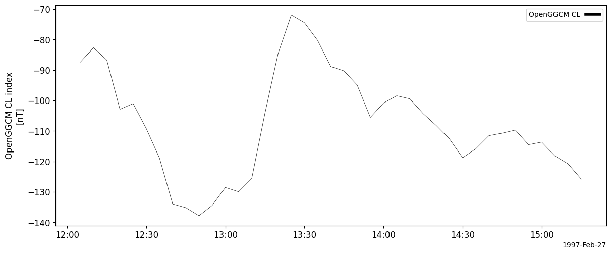
Calculating CL Index

cl = iof.ggcm.cl_index()
cl

<xarray.Dataset> Size: 624B
Dimensions:  (time: 39)
Coordinates:
  * time     (time) datetime64[ns] 312B 1997-02-27T12:05:00.170000 ... 1997-0...
Data variables:
    ggcm.cl  (time) float64 312B -87.42 -82.69 -86.71 ... -118.2 -120.8 -125.8

xarray.Dataset

• Dimensions:
  • time: 39
• Coordinates: (1)
  • time
    (time)
    datetime64[ns]
    1997-02-27T12:05:00.170000 ... 1...

    array(['1997-02-27T12:05:00.170000000', '1997-02-27T12:10:00.189000000',
           '1997-02-27T12:15:00.057000000', '1997-02-27T12:20:00.042000000',
           '1997-02-27T12:25:00.095000000', '1997-02-27T12:30:00.109000000',
           '1997-02-27T12:35:00.020000000', '1997-02-27T12:40:00.148000000',
           '1997-02-27T12:45:00.039000000', '1997-02-27T12:50:00.152000000',
           '1997-02-27T12:55:00.002000000', '1997-02-27T13:00:00.135000000',
           '1997-02-27T13:05:00.072000000', '1997-02-27T13:10:00.003000000',
           '1997-02-27T13:15:00.051000000', '1997-02-27T13:20:00.189000000',
           '1997-02-27T13:25:00.056000000', '1997-02-27T13:30:00.015000000',
           '1997-02-27T13:35:00.176000000', '1997-02-27T13:40:00.167000000',
           '1997-02-27T13:45:00.184000000', '1997-02-27T13:50:00.069000000',
           '1997-02-27T13:55:00.148000000', '1997-02-27T14:00:00.161000000',
           '1997-02-27T14:05:00.006000000', '1997-02-27T14:10:00.149000000',
           '1997-02-27T14:15:00.055000000', '1997-02-27T14:20:00.087000000',
           '1997-02-27T14:25:00.072000000', '1997-02-27T14:30:00.097000000',
           '1997-02-27T14:35:00.102000000', '1997-02-27T14:40:00.052000000',
           '1997-02-27T14:45:00.140000000', '1997-02-27T14:50:00.031000000',
           '1997-02-27T14:55:00.108000000', '1997-02-27T15:00:00.185000000',
           '1997-02-27T15:05:00.001000000', '1997-02-27T15:10:00.023000000',
           '1997-02-27T15:15:00.023000000'], dtype='datetime64[ns]')

• Data variables: (1)
  • ggcm.cl
    (time)
    float64
    -87.42 -82.69 ... -120.8 -125.8

    long_name :

    OpenGGCM CL index

    name :

    OpenGGCM CL

    units :

    nT

    array([ -87.41544377,  -82.69478258,  -86.71366913, -102.89215879,
           -101.02451853, -109.23313454, -118.88849372, -133.97621501,
           -135.18472031, -137.83206043, -134.44312685, -128.56528997,
           -129.95430154, -125.61871188, -104.25444685,  -84.60997947,
            -71.92627294,  -74.46922723,  -80.28978016,  -88.88048342,
            -90.30046755,  -94.94142006, -105.56266261, -100.85393853,
            -98.46431226,  -99.47876833, -104.28785657, -108.22649443,
           -112.61376187, -118.79556183, -115.87159321, -111.55128021,
           -110.7275196 , -109.70835973, -114.51247417, -113.67421848,
           -118.19346923, -120.80448641, -125.82781039])

• Indexes: (1)
  • time
    PandasIndex

    PandasIndex(DatetimeIndex(['1997-02-27 12:05:00.170000', '1997-02-27 12:10:00.189000',
                   '1997-02-27 12:15:00.057000', '1997-02-27 12:20:00.042000',
                   '1997-02-27 12:25:00.095000', '1997-02-27 12:30:00.109000',
                   '1997-02-27 12:35:00.020000', '1997-02-27 12:40:00.148000',
                   '1997-02-27 12:45:00.039000', '1997-02-27 12:50:00.152000',
                   '1997-02-27 12:55:00.002000', '1997-02-27 13:00:00.135000',
                   '1997-02-27 13:05:00.072000', '1997-02-27 13:10:00.003000',
                   '1997-02-27 13:15:00.051000', '1997-02-27 13:20:00.189000',
                   '1997-02-27 13:25:00.056000', '1997-02-27 13:30:00.015000',
                   '1997-02-27 13:35:00.176000', '1997-02-27 13:40:00.167000',
                   '1997-02-27 13:45:00.184000', '1997-02-27 13:50:00.069000',
                   '1997-02-27 13:55:00.148000', '1997-02-27 14:00:00.161000',
                   '1997-02-27 14:05:00.006000', '1997-02-27 14:10:00.149000',
                   '1997-02-27 14:15:00.055000', '1997-02-27 14:20:00.087000',
                   '1997-02-27 14:25:00.072000', '1997-02-27 14:30:00.097000',
                   '1997-02-27 14:35:00.102000', '1997-02-27 14:40:00.052000',
                   '1997-02-27 14:45:00.140000', '1997-02-27 14:50:00.031000',
                   '1997-02-27 14:55:00.108000', '1997-02-27 15:00:00.185000',
                   '1997-02-27 15:05:00.001000', '1997-02-27 15:10:00.023000',
                   '1997-02-27 15:15:00.023000'],
                  dtype='datetime64[ns]', name='time', freq=None))

• Attributes: (0)

ggcmpy.timeseries.store_to_pyspedas(cl["ggcm.cl"])
pyspedas.tplot("ggcm.cl")