Example: Tracing a Particle in a Dipole Field#

Here we use the BorisIntegrator as well, this time to calculate the trajectory of a gyrating particle in a dipole field similar to Earth’s.

The main new thing here is actually the use of discretized (gridded) electromagnetic field data.

Again, let’s start by importing some libraries. matplotlib and numpy are pretty universal. scipy.constants is for physical constants. Finally ggcmpy.tracing is where the tracing functionality currently lives.

pyvista is a library for (interactive) 3D visualization. It can be helpful to make sense of 3D trajectories, though those visualizations also could use more work still.

[1]:

from __future__ import annotations

import numpy as np
import pyvista as pv
import xarray as xr
from scipy import constants

import ggcmpy.tracing


def to_mesh_lines(df):
    positions = df[["x", "y", "z"]].to_numpy()
    mesh = pv.PolyData(positions)
    lines = pv.lines_from_points(positions)
    return mesh, lines


# utility function to plot trajectory using pyvista
def plot_trajectory(plotter, df, **kwargs):
    _, lines = to_mesh_lines(df)
    plotter.add_mesh(lines, **kwargs)


def plot_trajectories(plotter, dfs, **kwargs):
    for df in dfs:
        plot_trajectory(plotter, df, **kwargs)

Analytical and Discretized Dipole Field#

Let’s start by defining Earth’s dipole field (with the dipole being oriented straight North/South).

DipoleField just implements the analytic formula for a magnetic dipole.

[2]:

field = ggcmpy.tracing.DipoleField(m=np.array([0.0, 0.0, 8e22]))  # [A m^2]

Define a Grid#

Let’s define the coordinates of a simple grid extending from \(-10 R_E\) to \(R_E\). x, y, z are the cell centered coordinates – in OpenGGCM, that’s where the fluid quantities (density, pressure, velocity) live.

x_nc, y_nc, z_nc are the node-centered coordinates, ie., the actual boundaries of the computational cells.

[3]:

R_E = 6.371e6  # [m]
x = np.linspace(-10 * R_E, 10 * R_E, 20)
y = np.linspace(-10 * R_E, 10 * R_E, 20)
z = np.linspace(-10 * R_E, 10 * R_E, 20)
x_nc = 0.5 * (x[1:] + x[:-1])
y_nc = 0.5 * (y[1:] + y[:-1])
z_nc = 0.5 * (z[1:] + z[:-1])
coords = {"x": x, "y": y, "z": z, "x_nc": x_nc, "y_nc": y_nc, "z_nc": z_nc}

Set up Boris pusher parameters#

This is similar to how we set up the Boris pusher before in a uniform field. We again choose an electron, though it’s fudged to be really hot so one can see it’s gyration on the global scale. It is initialized at a distance of \(5 R_E\) in the equatorial plane.

[6]:

x0 = np.array([5.0 * R_E, 0.0, 0.0])  # [m]
B_x0 = field.B(x0)
T_e = 1.0 * 1e3 * constants.e  # 1 keV in J
v_e = np.sqrt(2 * T_e / constants.m_e)  # electron thermal speed
v_e *= 1000.0

om_ce = np.abs(constants.e) * np.linalg.norm(B_x0) / constants.m_e  # gyrofrequency
r_ce = constants.m_e * v_e / (constants.e * np.linalg.norm(field.B(x0)))  # gyroradius

v0 = np.array([0.0, v_e, v_e])  # [m/s]
print(f"B={B_x0} [T] om_ce={om_ce:.2f} [1/s] r_ce={r_ce / R_E:.2f} [R_E]")  # noqa: T201

t_max = 100.0 * 2 * np.pi / om_ce  # [s]
dt = 1.0 / om_ce / 10.0

B=[ 0.00000000e+00  0.00000000e+00 -2.47489717e-07] [T] om_ce=43528.99 [1/s] r_ce=0.07 [R_E]

Trace particle based on analytic dipole field#

[7]:

boris = ggcmpy.tracing.BorisIntegrator(field, q=-constants.e, m=constants.m_e)
df = boris.integrate(x0, v0, t_max)

Trace particle based cell centered discretized field#

[8]:

boris_cc = ggcmpy.tracing.BorisIntegrator(field_cc, q=-constants.e, m=constants.m_e)
df_cc = boris_cc.integrate(x0, v0, t_max)

Trace particle based Yee grid discretized field#

[9]:

boris_yee = ggcmpy.tracing.BorisIntegrator(field_yee, q=-constants.e, m=constants.m_e)
df_yee = boris_yee.integrate(x0, v0, t_max)

Trace particle based on Yee grid discretized field using Fortran#

This is the only variant that’s currently implemented in Fortran, as it’s hopefully the only one that’s really needed.

As one would hope, it is much faster.

[10]:

boris_f2py = ggcmpy.tracing.BorisIntegrator_f2py(
    field_yee, q=-constants.e, m=constants.m_e
)
df_f2py = boris_f2py.integrate(x0, v0, t_max, dt_max=dt)

Trace field lines#

[11]:

import pandas as pd
import scipy.integrate


def trace_field_line(r0, get_B, r_min=0.5, r_max=10.0):
    """Trace a magnetic field line starting at position r0 in the field
    provided by the get_B function.

    This function integrates the field line in the positive direction
    until it get either closer than `r_min` to the origin, or outside of `r_max`.

    Returns a pandas DataFrame with columns 'time', 'x', 'y', 'z'.
    """

    def rhs(t, x):  # noqa: ARG001
        B = get_B(x)
        B /= np.linalg.norm(B)
        return B

    def outside(t, x):  # noqa: ARG001
        return np.linalg.norm(x) - r_max  # stop if r > r_max

    outside.terminal = True
    outside.direction = 1  # only trigger when approaching from inside

    def inside(t, x):  # noqa: ARG001
        return np.linalg.norm(x) - r_min  # stop if r < r_min

    inside.terminal = True
    inside.direction = -1  # only trigger when approaching from outside

    tf = 1e9
    sol = scipy.integrate.solve_ivp(
        rhs, (0.0, tf), r0, events=[outside, inside], max_step=0.1 * R_E
    )
    sol2 = scipy.integrate.solve_ivp(
        rhs, (tf, 0.0), r0, events=[outside, inside], max_step=0.1 * R_E
    )
    dfs = [
        pd.DataFrame(np.column_stack((s.t, s.y.T)), columns=["time", "x", "y", "z"])
        for s in [sol, sol2]
    ]
    return pd.concat((dfs[1].iloc[::-1], dfs[0]), ignore_index=True)


def trace_field_lines(seeds, B_func, integrate_kwargs):
    """Trace multiple field lines.

    This is a convenience wrapper around trace_field_line.
    `seeds` is a list of starting positions.
    `B_func` is the magnetic field function.
    `integrate_kwargs` is a dictionary of additional keyword arguments to pass to
    `trace_field_line`.

    Returns a list of pandas DataFrames, one per seed point."""
    return [trace_field_line(r0, B_func, **integrate_kwargs) for r0 in seeds]


seeds = [
    r * np.array([np.cos(phi), np.sin(phi), 0.0])
    for phi in np.linspace(0.0, 2.0 * np.pi, 16, endpoint=False)
    for r in [3.0 * R_E, 5.0 * R_E]
]

dfs = trace_field_lines(
    seeds, field.B, integrate_kwargs={"r_min": 2 * R_E, "r_max": 20.0 * R_E}
)

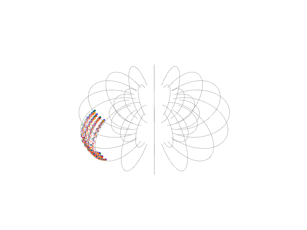
Plot the resulting trajectories#

All four trajectories describe the same physics, but numerically they are different because of the different ways the fields are provided / interpolated.

There are two implementations for the Yee grid discretized variant (Python and Fortran). These are green and orange, and one would hope for those two to agree – and they do.

[12]:

plotter = pv.Plotter()
plot_trajectory(plotter, df, line_width=1, color="blue")
plot_trajectory(plotter, df_cc, line_width=1, color="red")
plot_trajectory(plotter, df_yee, line_width=1, color="green")
plot_trajectory(plotter, df_f2py, line_width=1, color="orange")
plot_trajectories(plotter, dfs, line_width=1, color="gray")
plotter.show()

2026-02-18 23:11:03.821 (  59.728s) [    74239FC60B80]vtkXOpenGLRenderWindow.:1460  WARN| bad X server connection. DISPLAY=
/tmp/ipykernel_1557/1811996543.py:7: UserWarning: Failed to use notebook backend:

No module named 'trame'

Falling back to a static output.
  plotter.show()

Example: Tracing a Particle in a Dipole Field

Contents