Solar Wind Boundary Conditions#
Running the OpenGGCM runme will preprocess solar wind input data (either based on actual data, or a swdata file with synthetic solar wind conditions) and add it to the in.<run> file, which is read when actually running OpenGGCM and then used as the boundary condition for sunward boundary.
As part of the runme process, OpenGGCM will also generate a plot of these solar wind conditions, saved as swplot.<run>.satpl.ps. Since this is a postscript file, one may have to convert it before opening, e.g. using
$ ps2pdf swplot.cir07_19970227_liang_norcm.satpl.ps
$ open swplot.cir07_19970227_liang_norcm.satpl.pdf
OpenGGCM generally saves timeseries data in ASCII files, using a single file per quantity where each line has the the format YEAR MONTH DAY HOUR MINUTE SECOND.FRACTION VALUE.
ggcmpy supports reading those data files, and saving them as pyspedas tplot quantities, as demonstrated below.
Let’s start with some Python setup.
[1]:
from __future__ import annotations

import pyspedas

import ggcmpy
from ggcmpy.timeseries import (
    read_ggcm_solarwind_directory,
    read_ggcm_solarwind_file,
    store_to_pyspedas,
)
Reading a single timeseries file#
The function ggcmpy.timeseries.read_ggcm_solarwind_file() reads a single data file and returns it as a Pandas DataFrame.
Note: In the future, this function may change to return a xarray.DataArray instead, since this is what pyspedas uses internally, and it provides better support for attributes.
[2]:
df = read_ggcm_solarwind_file(
    ggcmpy.sample_dir / "cir07_19970227_liang_norcm/tmp.minvar/om1997.rr"
)
df
[2]:
| om1997.rr | |
|---|---|
| datetime | |
| 1997-02-27 10:00:00 | 2.22 |
| 1997-02-27 10:01:00 | 2.22 |
| 1997-02-27 10:02:00 | 2.21 |
| 1997-02-27 10:03:00 | 2.59 |
| 1997-02-27 10:04:00 | 1.99 |
| ... | ... |
| 1997-02-28 16:56:00 | 2.61 |
| 1997-02-28 16:57:00 | 2.51 |
| 1997-02-28 16:58:00 | 2.51 |
| 1997-02-28 16:59:00 | 2.53 |
| 1997-02-28 17:00:00 | 2.98 |
1861 rows × 1 columns
Reading multiple timeseries files from a directory#
You can also read all timeseries files from a directory using the read_ggcm_solarwind_directory() function. This function will return a Pandas DataFrame with multiple columns. In addition, using heuristics, attributes will be added naming the quantities and adding units.
[3]:
df = read_ggcm_solarwind_directory(
    ggcmpy.sample_dir / "cir07_19970227_liang_norcm/tmp.minvar", "om1997*gse"
)
df
[3]:
| om1997.vxgse | om1997.bygse | om1997.bzgse | om1997.vzgse | om1997.bxgse | om1997.vygse | |
|---|---|---|---|---|---|---|
| datetime | ||||||
| 1997-02-27 10:00:00 | -457.7 | -1.51 | -2.99 | -44.20 | 1.640 | 36.0 |
| 1997-02-27 10:01:00 | -457.7 | -1.51 | -2.99 | -44.20 | 1.640 | 36.0 |
| 1997-02-27 10:02:00 | -457.6 | -2.45 | -2.03 | -46.40 | 1.960 | 25.3 |
| 1997-02-27 10:03:00 | -438.1 | -2.08 | -1.68 | -36.00 | 2.270 | 11.9 |
| 1997-02-27 10:04:00 | -450.7 | -1.98 | -0.83 | -15.80 | 3.050 | 18.9 |
| ... | ... | ... | ... | ... | ... | ... |
| 1997-02-28 16:56:00 | -555.4 | -3.46 | -0.85 | -6.45 | 3.725 | -11.1 |
| 1997-02-28 16:57:00 | -551.1 | -2.97 | -1.20 | -12.30 | 4.030 | -12.8 |
| 1997-02-28 16:58:00 | -551.1 | -4.11 | -0.68 | -12.30 | 3.100 | -12.8 |
| 1997-02-28 16:59:00 | -550.9 | -4.31 | -0.69 | -12.70 | 2.890 | -11.4 |
| 1997-02-28 17:00:00 | -550.9 | -4.11 | -0.79 | -17.00 | 3.110 | 11.7 |
1861 rows × 6 columns
[4]:
df["om1997.bzgse"].attrs
[4]:
{}
Storing timeseries data in pyspedas#
The function store_to_pyspedas() will take a pandas DataFrame, as generated by the functions above, and store it as a pyspedas tplot variable for easy plotting:
[5]:
store_to_pyspedas(df)
pyspedas.tplot("om1997.bzgse")

ToDo: The function above does not yet automatically generate tplot vector variables. For now, one can use pyspedas to do so:
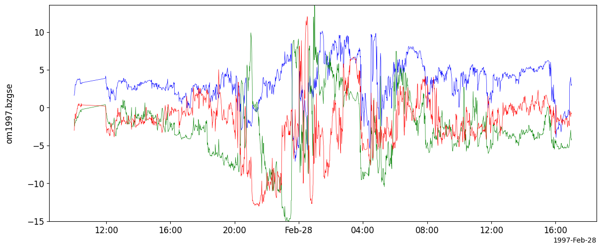
[6]:
pyspedas.options("om1997.bxgse", "color", "blue")
pyspedas.options("om1997.bygse", "color", "green")
pyspedas.options("om1997.bzgse", "color", "red")
pyspedas.store_data("om1997.bgse", ["om1997.bxgse", "om1997.bygse", "om1997.bzgse"])
pyspedas.tplot("om1997.bgse")